Option portfolio strategy

Markets are efficient and operate according to well-defined principles; they are not chaotic, though many people dive into this ocean without realising its true depth. Understanding the market is not as complicated as it may seem. At its core, the market is simply a place where transactions take place, enabling the transfer of ownership in businesses.

Among the various instruments available, there are tools designed to completely protect investments—these are called derivatives. In this article, I explain how such derivatives are used and the logic behind their design.

To give you a deeper, more practical understanding, I have shared my own real, live portfolio below. This will allow you to see the strategy in action. For clarity, I have also included a brief explanation of the concept behind this strategy before diving into the detailed portfolio breakdown.

This portfolio setup is totally risk free. Why risk free? because, we have purchased PUT option which completely eliminates the risk. immerse yourself for a complete understanding.

I have created a portfolio based on the principles of

• Black-Scholes model for option pricing.

• Put-call parity principle.

This portfolio is a simple arbitrage setup based on a Protective Collar Strategy. It is a simple, risk-free setup where capital is completely protected on the downside and profit is capped on the upside.

First, I will show my portfolio setup, its profit and loss report, and payoff graph, and I will explain the concepts and principles behind it.

three main things in this portfolio setup,

The first one, Principal investment.

There are three options.

1. Use cash to purchase assets, here Nifty ETFs or mutual funds.

2. Or be smart and use leverage instruments such as futures or options (only if you know how to use them)

3. Or a combination of futures, options, and ETFs

The choice is yours. I have used both ETF's, futures and options. for simplification i have shown only ETF's in the example.

Second, PUT option: to hedge investment on the downside, purchase a PUT option.

and third, a CALL option, which is used to offset the purchase cost of a PUT option.

Below is the live snapshot of my current portfolio.

Let me walk you through the portfolio I created on 1st January 2025 using a simple and powerful options strategy called the Protective Collar. It's designed to limit downside risk, while still giving decent upside — and the best part? The cost is almost negligible.

The minimum investment required is 70 lakhs, but better if invested 1 to 1.25 crore. This cash can be invested in risk free bonds, and can be kept as collateral. but as of now let's keep it simple.

What's in My Portfolio?

My portfolio has three main components:

1. Nifty ETF – Bought at ₹23,750

2. 24000 Strike Put Option – Bought at ₹812

3. 27000 Strike Call Option – Sold at ₹651

Let me explain why I chose these specific strikes and what they do.

Step-by-Step Breakdown

I Bought the Nifty ETF at ₹23,750

This is my core investment. I'm long on the market, and I want to benefit if Nifty goes up. But what if it falls? That's where the Put comes in.

I Bought a 24000 PUT at ₹812

This acts as my insurance. i have paid 812 per unit to purchase this,
No matter how far the market crashes, I have the right to sell my position at ₹24,000.
That means even if Nifty crashes to 20,000, or even below that level, my investment is protected. This limits my loss.

I Sold a 27000 CALL at ₹651

since i have purchased a PUT option by paying 812 from my hand, that's my max loss, inorder to cover the cost of purchasing the PUT at 24000, I sold a 27000 strike CALL Option.
This means if Nifty crosses 27,000, I’ll be forced to sell my ETF or investment at that price.
Yes, I cap my profits beyond 27K — but in return, I collect ₹651 upfront, which offsets most of the PUT’s cost.

What’s My Net Cost?

• PUT Premium Paid = ₹812

• CALL Premium Received = ₹651

• Net Cost = ₹812 - ₹651 = ₹161

So, my entire protection setup cost me just ₹161 per unit. That's almost nothing considering the peace of mind I get.

What’s My Max Loss?

Here’s the interesting part:
I bought the ETF at ₹23,750, but my PUT allows me to sell at ₹24,000.

That’s a built-in cushion of ₹250.

Even after accounting for the ₹161 cost, I’m still in profit if the market crashes.

[250-161 = 89. even market falls heavily i will still make money],

In short: my max loss is practically zero.

What’s My Max Profit?

I can benefit from the market rising all the way up to 27,000.
After that, the CALL I sold will be exercised, and I’ll be forced to sell at 27000.

So my max profit is:

₹27,000 - ₹23,750 - ₹161 = ₹3,089, rounded off, that’s a max gain of around 3,000 points.

I’m happy with that — solid upside and peace of mind on the downside.

Why I Like This Strategy,

This setup gives me:

• Low risk (almost no downside), zero loss

• Decent reward (maximum up to 3,000 points per unit), as per this model and my investment, maximum return is 75 lakhs per year.

• Fixed cost (₹161)

• Peace of mind — I’m protected, and I don’t have to worry about short-term volatility

I believe in managing risk first, and this strategy aligns perfectly with that mindset.

Below is the snapshot of Option chain taken on 31st July 2025. Just observe the price of CALL and PUT Option at Strike 25000, 29000.

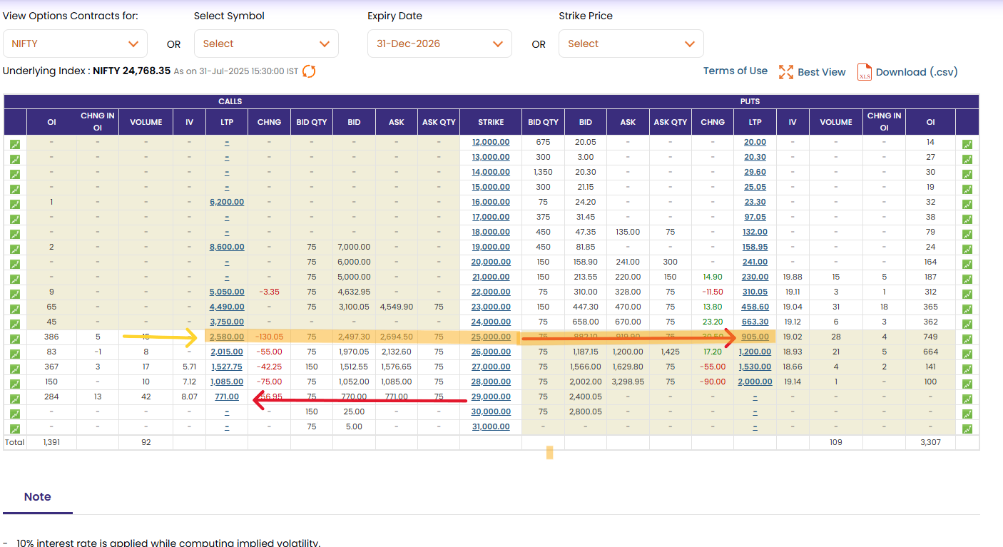
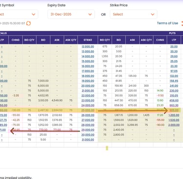
• You can notice Price of 25000 CALL Option is 2580,

• while Price of same strike 25000 PUT Option is just 905.

• And the price of 29000 CALL Option is 771.

I have explained why this disparity, just keep reading

Here shows a workflow for Selection of option contracts.

The most important task is to select the Strike or contracts of PUT options and CALL options.

Step 1. Check the price of Nifty Index.

Step 2. The PUT Option strike should be equal to or close to the spot price of the Nifty index.

For example, if the Nifty spot price is at 24900 or 24750, select a put option strike at 25000.

Step 3. Then check the price of the put option at the strike 25000. (in the example given above it is 905)

The price you pay to purchase PUT options is the cost of purchasing PUT option, which acts like insurance on the downside.

To offset the cost of purchasing put options,

Step 4: Select the CALL Option Strike Based on the PUT Option Price

Once you've bought the Put Option, the next step is to sell a CALL Option to offset the cost of the PUT. But how do you choose which CALL strike to sell?

Here’s a simple rule:

Look at the premium (price) you paid for the PUT Option, and then find a CALL Option Strike that is trading at approximately the same premium.

This ensures the income from selling the CALL roughly covers the cost of buying the PUT, creating a cost-effective protective collar.

Example:

• Nifty spot price is 24768 at the time of creating this portfolio

• You purchased a 25,000 PUT Option for ₹905.

• Now, go to the CALL side of the option chain and scan for the Call strike that is trading close to ₹905.

• You might find that the 29,000 CALL Option is trading around that price.

This means your maximum upside is capped at 29,000, but your protection on the downside is active below 25,000—and you've almost eliminated the net cost of the strategy.

Let’s look at this current setup:

• Nifty Spot Price: ₹24,750

• PUT Option (25000 strike): Bought at ₹905

• CALL Option (29000 strike): Sold at ₹770

The PUT Option I hold has a strike price of ₹25,000, but the market is currently trading at ₹24,750.

That means I have the right to sell Nifty at ₹25,000, while it’s only worth ₹24,750 in the market. That’s a direct value of:

₹25,000 - ₹24,750 = ₹250, This is called intrinsic value

So technically, my Put is already worth ₹250 more than the current spot — regardless of what the premium is doing. This is an unrealized gain, but a real edge.

• Put Cost: ₹905

• Call Premium Collected: ₹770

• Net Cost of Strategy: 905-770 = ₹135

Now subtract the current ₹250 intrinsic value of the Put from that:

Profit = ₹250 (intrinsic) - ₹135 (net cost) = ₹115 profit already. that means minimum guaranteed profit is 115, no matter in which direction market moves.

Now, the most important question arises, why such a difference?

Why is the price of a CALL option at strike 29000 equal to the price of a PUT option at strike 25000?

Why not Prices are equal at strike 25000?

What is the reason for it?

The answer lies in the Black-Scholes model and PUT-CALL parity principle.

In this model, The loss is zero, and the maximum profit is capped at 3000 points. (27000-24000). This is the difference in the strike of the CALL option and the PUT option, which makes maximum gains. But is it that simple, really? It must be some mistake; this can't be true. Isn't it?

Well, everything is perfect here; everything is following a set of principles. The market is always efficient; it doesn't create the arbitrage opportunity easily, but this is not an arbitrage. This pricing is done purely on the basis of the Black-Scholes model, and here all mathematical models are perfectly intact. No rules broken.

Before we move on, keep these 3,000 points in mind — and stay with me, because I’ll reveal why the limit is exactly 3,000 at the very end.

Let's Understand the concept in terms of a real estate analogy.

In order to understand this model, let me explain using an example of Real Estate and Gold.

Say, You have invested in a Real Estate property. You purchased a plot worth ₹1 crore, and now you want to sell it to make some gains. You plan to sell it at a price of ₹1.25 crores (₹1,25,00,000). You find a buyer who is interested in the property and agrees to your asking price—but he requests to pay the entire amount after one year.

What would you do in this situation? Think for a while…

Done?

Okay—now think: What if, after one year, he’s no longer interested in purchasing the property?
To avoid that uncertainty, you make an agreement with the potential buyer by taking an advance payment—say ₹5 lakhs. If the buyer backs out and shows no interest in going ahead with the deal, you get to keep that advance amount. On the other hand, if he honors the agreement, you are obligated to sell him the property at the agreed price—even if the market price has gone above ₹1.25 crores.

In this situation, you are locking in a profit of ₹25 lakhs.

This advance amount received works exactly like the call option premium you receive when selling a call option at a strike of 28,000 in our Nifty portfolio model.

In simple terms:
You're agreeing to sell your Nifty investment at a price of 28,000, after one year, and in return, you're receiving a premium of ₹800 per share.

Scenario 1: Land price stays at ₹1 crore or drops to ₹90 lakhs

Potential Buyer doesn’t exercise his option. You keep your land. When price is 1 crore or less why will he buy from you for 1.25 Crores.

• And the ₹5 lakhs? You keep it as income.

• So, your profit = ₹5 lakhs

Scenario 2: Land price rises to ₹1.4 crore

Potential Buyer exercises his CALL Option and buys your land at ₹1.25 crore.

• You must sell it to him, even though it’s worth more

• You receive ₹1.25 crore + ₹5 lakhs (premium)

• But the market value is ₹1.4 crore

• You miss out on ₹40 lakhs of gain, effectively losing ₹15 lakhs of potential profit, your overall profit is still 25 Lakhs

This is your opportunity cost

So Why Sell Call Options at All?

Because:

• You want some immediate income (the ₹5 lakhs upfront)

· You want to cover the cost of purchasing insurance for the property, to protect the cost of purchasing.

• You believe prices won’t rise much

• You’re okay selling the asset at the agreed price

• You already own the asset—so you're just making money while holding it
  (this is called a covered call strategy)

Connecting Back to the Stock Market

In your Nifty collar strategy, you're doing the same thing:

• You own Nifty (through ETF/futures) purchased at the price of 24000.

• You sell a call at a higher strike price (say 27,000)

• You collect the premium (say ₹800)

• Even if Nifty rises above 27,000, you're committed to sell—but you've already locked in profits

But if you're combining this with a PUT (like in your protective collar) — then you’re simply creating a price band: limited downside, limited upside, and full capital protection.

Now lets understand on the pricing of the PUT option.

Imagine you own 100 grams of Gold.

Let’s say the current market price of Gold is ₹10,000 per gram, so your Gold is worth:

₹10,000 × 100 grams = ₹10,00,000

You’re worried that Gold prices might fall in the next few months, but you don’t want to sell it right now. Maybe it's an investment, maybe it's family Gold, or maybe you're waiting for the right time to sell.

So what do you do?

You go to a jeweler or financial institution and make an agreement:

You pay them ₹20,000 today (this is premium you are paying), and in return, they promise to buy your gold at ₹10,000 per gram any time in the next 12 months—even if the market price drops.

This agreement is exactly what a PUT option is.

You’re buying the right to sell your Gold at a fixed price.

Scenario 1: Gold price falls to ₹7,500 per gram

• Now your Gold is worth ₹7,50,000

• But you have the right to sell it for ₹10,00,000

• You use your put option and sell at ₹10,00,000

• You make ₹250,000 profit (₹10,00,000 − ₹7,50,000)

• Subtract the ₹20,000 premium you paid

• Net profit = 250,0000 – 20,000 = ₹230,000

You protected yourself from the fall in gold prices!

Infact this is not a profit, since you have purchased the Gold by paying lakhs, even if it is worth 7,50,000 today, you still retain its buying value. Your maximum loss is 20,000, which is the cost of purchasing insurance on the downside.

Scenario 2: Gold price goes up to ₹11,500 per gram

• Your Gold is now worth ₹11,50,000

• You simply don’t use the option

• You sell the gold at market price and earn full profit

• You lose only the ₹20,000 premium you paid

You still make profit, just minus the small insurance cost.

A PUT option is like insurance:

• You pay a small premium today

• In return, you get the right to sell your asset at a fixed price

• If the price falls, your value is protected

• If the price rises, you ignore the insurance and enjoy the gain

Just like you buy insurance for your house, health, or car—you buy a PUT option to protect your investment (whether it’s gold, Nifty, or a stock).

Tying It All Together — The Protective Collar Strategy

Now, let’s combine both ideas.

In our portfolio, you hold Nifty ETFs or a Nifty futures position.

• You buy a PUT option to protect against downside loss (just like the gold insurance).

• You sell a CALL option to earn a premium and offset the cost of the PUT options (just like the advance on the property deal).

This combination is called a Protective Collar Strategy.

It’s a setup where:

• Your downside is protected.

• Your upside is capped.

• But you have no net cost, or even a small credit.

You’re giving up unlimited upside in exchange for peace of mind—a safe, limited-risk profile.

So the question now arises: why is the premium ₹800? Why not less or more?
Or, in terms of the Real Estate story: why did you agree to ₹5 lakhs only as the advance amount?

Imagine this: if you had sold the property today and deposited that money in a bank, it could have earned you a risk-free interest rate of 5%—which amounts to ₹5 lakhs in a year. Since the buyer is deferring the payment by one year, you have the right to demand that ₹5 lakhs upfront as an advance. Even if he dishonors the agreement, you still get to keep that ₹5 lakhs. That covers your loss of purchasing power over time due to inflation.

The risk-free interest rate exists for exactly this reason: to protect the purchasing power of money over time. Of course, institutions like banks and governments are better positioned to manage this—why?
To understand that, you can read on inflation-induced debt destruction. Which is on the other side of the blog.

In our case, this ₹5 lakh advance (or the ₹800 option premium) is not random. It reflects a combination of several key financial principles, including:

• Time value of money

• Inflation

• Risk-free interest rate

All of these are fundamental components in the Black-Scholes Model for pricing options.

Let’s say today’s Nifty ETF price is ₹25,000, and the risk-free interest rate is 10% per year.
Naturally, over a year, you'd expect ₹25,000 to grow by 10%, reaching ₹27,500. That’s a 10% return from a risk-free investment, like a government bond.

Options Are Priced on the Expected Future Value — Already Discounted

In options theory (specifically the Black-Scholes model), the price of an option reflects the present value of future expectations. The ₹2,500 increase due to 10% interest is already priced into the market via the forward price of the Nifty — but options are priced under risk-neutral probabilities, not real-world probabilities.

The market assumes:

"If Nifty is ₹25,000 today and the risk-free rate is 10%, then the forward value of Nifty after one year should be ₹27,500. So that becomes our base expectation."

Let’s assume the current Nifty price is ₹25,000, and the risk-free interest rate is 10% annually. Over one year, this implies a natural price growth of ₹2,500, meaning the expected forward value of Nifty is ₹27,500.

Now, consider a Call Option with a strike price of 27,000.

This strike is already ₹2,000 above the current spot price (27,000 - 25,000 = 2,000). Based on the 10% growth expectation, the market believes Nifty may reach around 27,500 in a year — which is just ₹500 above the strike price.

That extra ₹500 is the expected intrinsic value of the CALL Option at expiry. But options aren't just about intrinsic value — their prices also include time value, implied volatility (IV), and theta (time decay).

These additional factors explain why the premium is ₹800, not just ₹500. The market is pricing in the probability that Nifty may go even higher than 27,500, or that it may reach there sooner than expected, giving the Call Option extra value beyond its basic forward calculation.

Black Scholes Model for option pricing

Options are priced based on the Principle of Black Scholes Model. In this section i will answer all the questions raised earlier.

The Black-Scholes Model is fundamentally based on the concept of time value of money — the idea that a rupee today is worth more than a rupee tomorrow.

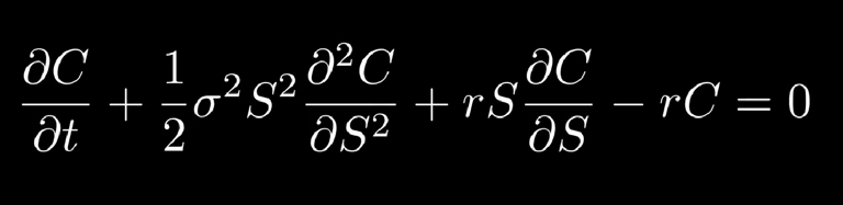
The Black–Scholes Model

As I mentioned earlier, in the previous section where I explained the constituents of my portfolio, I noted that I would also explain in detail why the calculation of CALL and PUT options was necessary. Let us now see why this is important.

To understand this, we need to briefly go back in history. I will not go into too much detail, but only highlight some key points. In those earlier days, there was no proper theory or framework to calculate the price of CALL and PUT options. Everyone used their own methods of calculation. As trade in goods and services expanded, the need for a standardized framework became essential.

One early attempt came from a study, which modeled prices based on randomness of movement, inspired by the motion of physical particles.

Early Methods of Option Pricing

• Louis Bachelier (1900)
  Bachelier was the first person to try and mathematically value options. In his PhD thesis, he imagined stock prices moving randomly—sometimes up, sometimes down—just like particles moving in water.
  He called this a random walk. Using this idea, he built formulas to estimate the “fair price” of an option.
  His work was ahead of its time and not widely used back then, but it laid the foundation for modern finance.

• Brownian Motion Connection
  Around the same time, physicists like Einstein were studying how tiny particles jiggle around when suspended in liquid. This motion is called Brownian motion.
  Surprisingly, the math behind Brownian motion turned out to be almost the same as the math behind Bachelier’s random walk for stock prices.
  This link gave finance a strong scientific basis: if particles move randomly but still follow mathematical patterns, maybe stock prices do too.

However, Black and Scholes were not convinced by this model, since stock prices are not purely random. They move according to factors such as company profits, growth, and broader market conditions. It was not absolute randomness.

Bachelier imagined stock prices moving like random steps, much like how particles bounce around in water. This was the first step toward option pricing models, and later, the Black-Scholes model refined it into the version used today. Black and Scholes accepted the concept of randomness, but framed it within a risk-neutral world.

Developed by Fischer Black, Myron Scholes, and Robert Merton in the early 1970s, the Black–Scholes model was a breakthrough in modern finance. It provides a closed-form solution for pricing European options by considering:

• The current asset price

• The strike price of the option

• The time to expiration

• The risk-free interest rate

• The volatility of the asset’s returns

A key insight is that if risk is completely eliminated—for instance, by holding a fully hedged position—the return on that position should be no greater than the risk-free rate (e.g., government bond yield). Otherwise, arbitrage opportunities would exist, allowing traders to earn profits without taking risk.

While Bachelier’s random walk idea was revolutionary, it had some flaws. For example, his model sometimes gave stock prices that could go below zero, which isn’t realistic.

When Black and Scholes were developing their model, they faced a criticism:
Stock prices aren’t truly random. They move for reasons — company profits, economic changes, news, interest rates, and so on. Compared to dice rolling, markets have patterns, reactions, and human behavior.

The Core Logic Behind Black–Scholes

When Black and Scholes developed their model for pricing options, they relied on a few key ideas:

1. Efficient Markets (EMH):
   Markets are generally efficient, meaning prices quickly reflect available information. In such a market, option prices shouldn’t allow traders to make “easy money.”

2. No Arbitrage Principle:
   At any given moment, option pricing must not create arbitrage opportunities. If arbitrage exists, it’s essentially free money.

3. Risk-Free Interest Rate:
   The model assumes that the benchmark for “safe” returns is the risk-free interest rate (like government bonds). When an option is properly hedged the risk is removed. With the risk is totally Removed The maximum profit investor should make is a risk free return, Price of put auction and call option should be determined in such a way that it should not give more returns than fixed returns instruments like Fixed deposits or govt securities or govt bonds.

4. Pricing Balance:
   The model also reflects natural market behavior. If option prices are too low, everyone will rush to buy them. If prices are too high, nobody will touch them. The Black–Scholes framework balances these forces, keeping option prices in a “fair zone” where supply and demand meet.

In essence: Instead of trying to predict uncertain future returns, the Black–Scholes model anchored option prices to something stable and universal—the risk-free rate. This shift was the breakthrough that made large-scale option trading possible.

In the Indian stock market, the risk-free rate is generally assumed to be 10% when calculating option prices.

Why 10%?
If the risk-free interest rate is set higher, the price of a call option will also be higher, and very few people would be willing to buy it. On the other hand, if the risk-free interest rate is set too low, the call option price will be very cheap, and everyone would rush to buy it.

In practice, the average return from the Nifty index is usually more than 12%. So, when compared to that, taking a 4% risk is considered manageable. That’s why the risk-free rate is taken as 10% in option pricing.

CALL - PUT Parity

what this duggests that, at any oint of time, the return on the option shouldnot b emore than risk free interest rate